Introduction
Composer and research scientist Jean-Claude Risset's harmonic arpeggio instrument produces a beautiful drone-like sound, over which occurs a downward cascading arpeggio of a composer-specified subset of the harmonic series. The instrument's timbre is likened by some to the sound produced by an overtone singer. Created by beating patterns that result from closely-spaced sinusoids, Risset describes the arpeggio gestures as "spectral scans" [1]. "Risset's arpeggio" is a perfect vehicle for exploring Risset's interest in creating instruments that are sonic processes and are capable of producing rich timbres that respond predictably under precise parametric control. What is more, the instrument is a convenient entry point into the worlds of spectral composition and sine wave interference patterns. Inspired by Risset's amazing instrument, the author employed similar designs in his Csound composition Strange Attractors & Logarithmic Spirals (2001) [2]. This article introduces Risset's instrument and then presents some compositional examples that demonstrate how the author extended it for use in his aforementioned composition.
Download the Code Example Files: BainRissetArpeggioEx.zip
Note: This article uses a Greek letter that may not correctly display in some browsers. If the Greek capital letter delta is not displayed here: Δ, please try another browser like Mozilla, Opera, Safari, etc. that supports the use of this character.
I. The Arpeggio Instrument
Historical Background
Risset's arpeggio is one of the examples presented in his "Introductory Catalogue of Computer Synthesized Sounds," a collection of timbres and sonic processes that he created at Bell Telephone Laboratories [3]. He assembled this collection in 1969 for one of the first computer music courses at Stanford University [4]. Originally coded in MUSIC V, Csound versions of the instruments are currently available to the reader in the The Csound Catalog with Audio CD-ROM [5] and Amsterdam Catalogue of Csound Computer Instruments (ACCCI) [6]. Finally, it should be mentioned that the arpeggio instrument is prominently featured in Risset's compositions Inharmonique (1977), Songes (1979) and Contours (1982) [7].
Csound Code Examples and Prerequisites
This article has seven downloadable code example files (see the .zip file above). These example files are referred to in the article and should be rendered using Csound so that the audio examples may be heard. Example 1 shows the Csound code for Risset's arpeggio that is used in the first code example file and in the discussion that follows.
sr        =         44100
kr        =         4410
ksmps     =         10
nchnls    =         1

          instr 10

idur      =         p3
ifreq     =         p4
iamp      =         p5
ideltaf   =         p6
irise     =         p7
idecay    =         p8
iwf       =         p9

i1        =         ideltaf
i2        =         2*ideltaf
i3        =         3*ideltaf
i4        =         4*ideltaf

aenv      linen     iamp,irise,idur,idecay

a1        oscili    aenv,ifreq,iwf

a2        oscili    aenv,ifreq+i1,iwf
a3        oscili    aenv,ifreq-i1,iwf

a4        oscili    aenv,ifreq+i2,iwf
a5        oscili    aenv,ifreq-i2,iwf

a6        oscili    aenv,ifreq+i3,iwf
a7        oscili    aenv,ifreq-i3,iwf

a8        oscili    aenv,ifreq+i4,iwf
a9        oscili    aenv,ifreq-i4,iwf

          out       a1+a2+a3+a4+a5+a6+a7+a8+a9

          endin
(a)
;             1  2  3  4  5  6  7  8  9  10
f1  0 4096 10 1  0  0  0  .7 .7 .7 .7 .7 .7

;   st idur ifreq iamp ideltaf irise idecay iwf
i10 0  7    96    2100 .03     .02   .5     1
e
(b)
Example 1. Risset's arpeggio: (a) orchestra code and (b) score code.
The reader should be aware that the code presented in Example 1 differs from Risset's original instrument and is based on the Csound code published in The Csound Catalog. Readers in need of a canonical version of the Csound code for Risset's instrument should consult The Csound Catalog or the ACCCI versions cited above. Finally, it should be mentioned that a basic knowledge of the harmonic series and Csound syntax is assumed below. Readers in need of a Csound tutorial for beginners should consult Richard Boulanger's Introduction to Sound Design in Csound, Chapter 1 of the The Csound Book, which is available in print and online [8].
Controlling the Pitch Content of the Arpeggio
We begin our discussion of Example 1 with the score code's f-statement. As shown in Figure 1, GEN10 [9] is used to create a composite waveform built from the weighted sum of seven sinusoids.
;            1  2  3  4  5  6  7  8  9  10
f1 0 4096 10 1  0  0  0  .7 .7 .7 .7 .7 .7
Figure 1. GEN10 controls the pitch content of the harmonic arpeggio.
The comment statement (;) numbers the harmonic partials of GEN10. The frequency relationships in the GEN10 specification are:
f, 5f, 6f, 7f, 8f, 9f, and 10f,
where f is the fundamental frequency [10]. To obtain the actual frequencies of the seven sinusoidal components, multiply the respective partial numbers by the fundamental frequency (ifreq) given in the i-statement in Figure 2.
;   st idur ifreq iamp ideltaf irise idecay iwf
i10 0  7    96    2100 .03     .02   .5     1
Figure 2. The i-statement specifies the fundamental frequency, as well as other parameters.
The seven frequencies specified by the GEN10 routine in Figure 1 are:
96, 480, 576, 672, 768, 864 and 960 Hz,
whose relative amplitudes are
1, 0.7, 0.7, 0.7, 0.7, 0.7 and 0.7,
respectively. In Figure 1, be sure to note that partial 1's amplitude value is set to 1 (giving it some extra weight) whereas partials 5, 6, 7, 8, 9 and 10 are all set to the same lesser value 0.7. Note too how partials 2, 3 and 4 are omitted by setting their values to 0. The GEN10 routine sums these seven sinusoids and creates the requested 4096-point function table (f-table) f1 which loads at time 0 [11]. Figure 3 shows one cycle of f1's waveform alongside its spectrum [12].
|
|
|
|
(a) |
(b) |
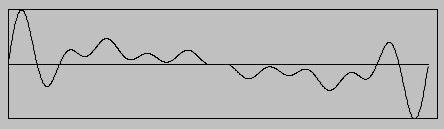
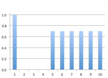
Figure 3. F-table 1 (f1): (a) Waveform (amplitude vs. time) and
(b) Spectrum (relative amplitude vs. harmonic partial number).
We will refer to the waveform/spectrum stored in the f-table as the source spectrum because, as we will soon see, it controls the pitch content of Risset's arpeggio.
GEN10 is an ideal tool for creating composite waveforms from harmonically-related sinusoidal components that have static amplitudes. For example, the f-statement in Figure 4 generates f-table 2 (f2), a source spectrum based on the first 16 partials of the harmonic series, in a single line of code.
;            1 2 3 4 5 6 7 8 9 10 11 12 13 14 15 16
f2 0 4096 10 1 1 1 1 1 1 1 1 1 1  1  1  1  1  1  1
Figure 4. F-table 2 (f2): a function table created using partials 1-16 of the harmonic series, inclusive.
Notice that, unlike the partial configuration in Figure 1, all of the partials here are equally weighted. To emphasize certain partials over others the relative amplitude values of the GEN10 routine must be strategically weighted. For composers interested in exploring the harmonic and linear resources implied by harmonic series proportions, it may be useful to think of the series in terms of traditional music notation. Since 96 Hz is approximately the pitch G2 (C4 is middle C), we show the series on that fundamental pitch in Figure 5.
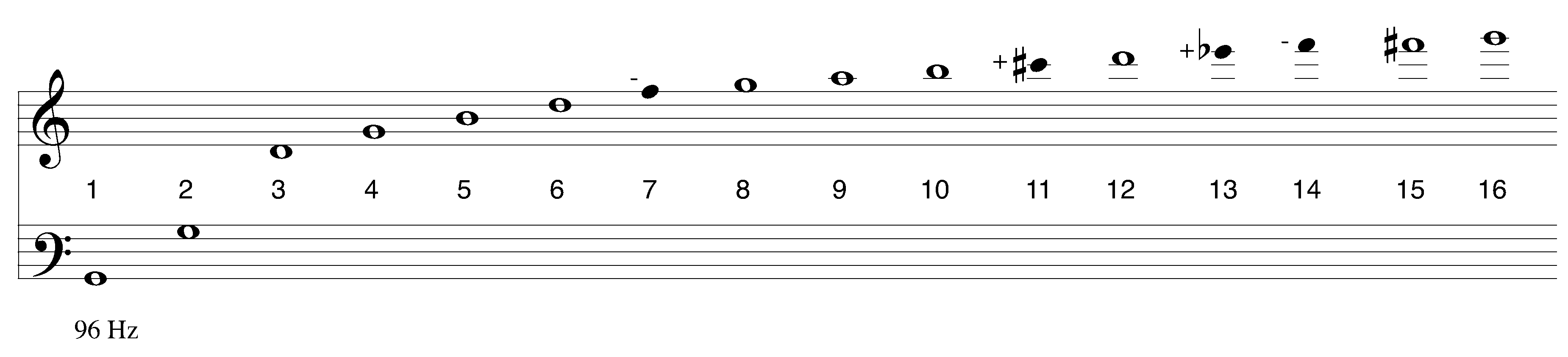
Figure 5. Traditional music notation for the first 16 partials of the G2 harmonic series.
The noteheads of partials 7, 11, 13, and 14 are filled in because their tunings are significantly different (lower or higher, respectively) than their equal-tempered counterparts. Of course, the harmonic series contains an infinite number of possibilities for compositional exploration. Two interesting examples include the 6:5:4 just major triad
f3 0 4096 10 0 0 0 1 1 1
stored in f3, and the natural scale created from partials 8-16 (with partial 14 omitted) stored in f4.
f4 0 4096 10 0 0 0 0 0 0 0 1 1 1 1 1 1 0 1 1
Rendering code example file "1-RissetArpeggio.csd" using Csound, we can hear Risset's arpeggio of source spectrum f1, as well arepeggios of f2, f3 and f4.
When f1 is the source spectrum, Risset's harmonic arpeggio sounds something like the gesture notated below in Figure 6.
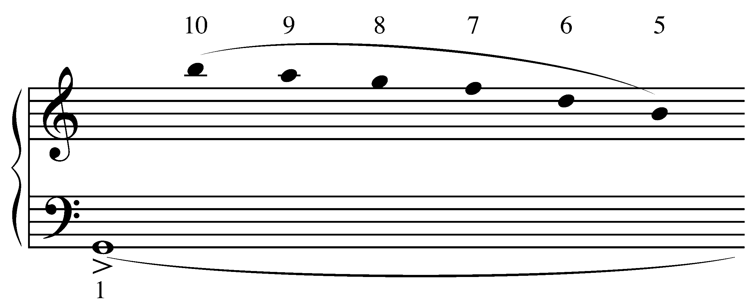
Figure 6. Chantlike music notation approximating the first seven seconds of
the arpeggio of source spectrum f1.
Although this chantlike notation (with harmonic partial numbers) can convey the basic pitch sequence for the first few seconds of the arpeggio, it is difficult to notate the gesture over longer time spans. One remarkable feature of Risset's arpeggio is the heavily accented attack phase of the tone. This is caused by the phase relationships between its constituent parts. In order to get a better sense of the range of possibilities that may be explored, we need to gain a better understanding of how this instrument exploits wave interference patterns between slightly mistuned digital oscillators to create such beautiful, and intricately-woven, musical fabrics.
Instrument Design
Charles Dodge and Thomas Jerse provide an analysis of Risset's instrument in their book Computer Music: Synthesis, Composition, and Performance [13]. The authors discuss the instrument's appearance about 3 minutes into Risset's composition Inharmonique, describing its sonic quality as dronelike with a clearly perceived fundamental, over which occurs a downward cascading arpeggio through the harmonic series. Looking at Example 1 (a) again, we can see that nine interpolating oscillators (oscili) create this dynamic timbre. All nine oscillators share the same amplitude envelope (aenv), phase (0) and composite waveform (iwf), however, each oscillator is tuned to a slightly different fundamental frequency. As Figure 7 shows, the frequency offset variables evenly space the fundamental frequencies symmetrically above and below ifreq.
Audio signal: |
a9 |
a7 |
a5 |
a3 |
a1 |
a2 |
a4 |
a6 |
a8 |
|
Fund. freq.: |
ifreq-i4 |
ifreq-i3 |
ifreq-i2 |
ifreq-i1 |
ifreq |
ifreq+i1 |
ifreq+i2 |
ifreq+i3 |
ifreq+i4 |
|
95.88 |
95.91 |
95.94 |
95.97 |
96.00 |
96.03 |
96.06 |
96.09 |
96.12 |
Hz |
Figure 7. Fundamental frequencies of the nine oscillators when ifreq = 96 Hz and i1 = 3/100 Hz.
In total, 63 sinusoids are interacting to create the arpeggio of f1. For source spectrum with n sinusoidal components, 9n sinusoids are interacting to create the arpeggio. Because the frequency offsets are all expressible in terms of i1, Figure 8 shows one way to view Risset's instrument: as the source spectrum (ss) applied to each of the nine symmetrically mistuned fundamental frequencies.
a9 |
a7 |
a5 |
a3 |
a1 |
a2 |
a4 |
a6 |
a8 |
ss(ifreq-4i1) |
ss(ifreq-3i1) |
ss(ifreq-2i1) |
ss(ifreq-i1) |
ss(ifreq) |
ss(ifreq+i1) |
ss(ifreq+2i1) |
ss(ifreq+3i1) |
ss(ifreq+4i1) |
Figure 8. The source spectrum (ss) applied to each of the nine symmetrically mistuned fundamental frequencies.
The Beating Effect
When two sinusoids with slightly different frequencies (and with equal amplitudes and phases) are summed, the result is an interference pattern called first-order beats, or more informally beats [14]. Beats are the periodic variation we perceive in the amplitude of the resultant tone. Most musicians are familiar with this beating effect from the traditional role it plays in tuning instruments. A bit of trigonometry, however, is required to describe the phenomenon precisely. Say the frequencies of the two sinusoids we want to mix (see the + sign in equation 1, below) together in Csound are f1 and f2 (each sinusoid with amplitude 1 and phase 0), the resultant waveform may be described by equation (1).
|
(1) |
Using a standard trigonometric identity we get equation (2) [15].
|
(2) |
Equation (2) shows that the linear superposition of the two sine waves in equation (1) is another sine wave whose frequency is the average of the two original frequencies and whose amplitude is modulated (see the * sign in equation 2, above) by a cosine wave. The average of the two frequencies, (f1+f2)/2 in equation (2), is called the center frequency. The periodic variation in the amplitude of the resultant tone is caused by the cosine wave. The number of variations per second we perceive, called the beat frequency (Δf), is equal to the difference between the two frequencies. Note that it matters not whether f1 is greater than f2, or f2 is greater than f1. Equation (3) shows a concrete example, the sum of two sub-audio sinusoids (f1 = 1 Hz, and f2 = 1.1 Hz) whose frequencies are close and whose amplitudes have been scaled by 1/2 so that the peak amplitude of the resultant waveform is 1.
|
(3) |
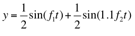
Figure 9 (a) shows the graph of the destructive interference pattern created by equation (3).
|
|
|
(a) |
(b) |
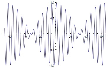
Figure 9. Beats.
Figure 9 (b) shows the same graph with the cosine "amplitude envelope" outlined. Rendering code example file "2-Beats.csd" using Csound, we can explore a wide variety of beat patterns. For example, 440 and 442 Hz sinusoids produce 2 beats per second; as do 440 and 438 Hz. (i.e., Δf= 2); 440 and 443 Hz produce 3 beats per second, as do 440 and 437 Hz (Δf= 3); and so on. Experimenting with frequency separations less than1 Hz:440 and 440.1 Hz produces 1 beat every ten seconds (Δf= 1/10); 440 and 440.2 Hz produce 2 beats every ten seconds, which simplifies to 1 beat every 5 seconds (Δf= 2/10 = 1/5); and 440 and 440.08 produce 8 beats every 100 seconds, which simplifies to 2 beats every 25 seconds (Δf= 8/100 = 2/25); and so on. Be sure to experiment with a wide variety of values for f1 and Δf.
Finally, it is important to understand that at a certain frequency separation, the beating sensation gives way to a sensation of roughness. At a still larger separation, two separate tones are perceived. We can explore this continuum of sensations by holding f1 constant and slowly moving f2 away from it in either direction. Code example file "2-Beats.csd" also contains a simple tone experiment that holds f1 constant at A4, 440 Hz. while f2 glissandos exponentially from: (1) 440 to 660 Hz, up a 3:2 fifth; and (2) 440 to 293.333 Hz , down a 3:2 fifth. First we hear a unison, followed by beats, then we experience a sensation of roughness, and ultimately two separate tones (not to mention combination tones). When Δf is less than about 10-15 Hz we typically hear the beating effect, but keep in mind the exact value depends on frequency.
Controlling the Rate of the Arpeggio
Rendering code example file "3-ArpeggioRate.csd" using Csound we can explore how ideltaf, or i1, affects the rate of the arpeggio for a given source spectrum. In general, the larger the value of ideltaf the faster the rate of the harmonic arpeggio. Values less than about 1/10 Hz are typically useful.
To understand why Risset's instrument produces the downward cascade of the source spectrum's component frequencies, it is helpful to create a 7 x 9 matrix of all the frequencies involved [16]. Furthermore, if we set ifreq and ideltaf to convenient values, it is much easier to see the harmonic partial and beat frequency relationships. For example, if we set ifreq to 100.4 and ideltaf to 0.1 Hz we get the following convenient set of nine mistuned fundamentals:
S= {100, 100.1, 100.2, 100.3, 100.4, 100.5, 100.6, 100.7, 100.8}.
Applying source spectrum f1 to the nine members of S, we get the 63 frequencies shown in Figure 10.
nS |
|||||||||
S |
100 |
100.1 |
100.2 |
100.3 |
100.4 |
100.5 |
100.6 |
100.7 |
100.8 |
5S |
500 |
500.5 |
501 |
501.5 |
502 |
502.5 |
503 |
503.5 |
504 |
6S |
600 |
600.6 |
601.2 |
601.8 |
602.4 |
603 |
603.6 |
604.2 |
604.8 |
7S |
700 |
700.7 |
701.4 |
702.1 |
702.8 |
703.5 |
704.2 |
704.9 |
705.6 |
8S |
800 |
800.8 |
801.6 |
802.4 |
803.2 |
804 |
804.8 |
805.6 |
806.4 |
9S |
900 |
900.9 |
901.8 |
902.7 |
903.6 |
904.5 |
905.4 |
906.3 |
907.2 |
10S |
1000 |
1001 |
1002 |
1003 |
1004 |
1005 |
1006 |
1007 |
1008 |
a9 |
a7 |
a5 |
a3 |
a1 |
a2 |
a4 |
a6 |
a8 |
Figure 10. 7 x 9 frequency matrix for ifreq = 100.4 Hz and ideltaf = 1/10 Hz.
Rendering code example file "4-Fig10Matrix.csd" using Csound, we can hear each row of the matrix presented in high-to-low order (i.e., 10S, 9S, 8S, etc.), first individually, then superposed one at a time until all rows are sounding together. (It should be mentioned that unlike in Example 1, this example uses 63 equally-weighted sinusoids.) When the rows are played individually, be sure to note the distinct interference pattern created by each row. When they are superposed, be sure to note how Risset's arpeggio slowly begins to emerge as each row of the matrix is added. The relative rates at which the rows reach peak amplitude might be described as a 10:9:8:7:6:5:1 polyrhythm. The differing rates cause the members of the f1 source spectrum (represented by the rows of the matrix) to come into phase in descending order, creating the downward cascading effect. For longer durations, a macro-level textural "phasing" effect becomes apparent that is similar to the resultant patterns found in the phase music of American composer Steve Reich [17].
To gain an even deeper appreciation for the complexity of the beating effect, consider that each row of Figure 10 actually produces 36 first-order beating pairs of sinusoids. This is the number of 2 element combinations created by each 9-tone row [18]. If second-order beats (e.g., beats between octave-related sinusoids) and binaural beats (beats between sinusoidal pairs presented separately to the left and right ears) are taken into account, there are even more possibilities to consider.
II. Strange Attractors & Logarithmic Spirals
Extending Risset's Instrument Design
The author's Csound composition Strange Attractors & Logarithmic Spirals sets two beautiful mathematical forms into opposition: strange attractors, chaotic systems that cycle periodically, yet never repeat exactly the same pattern; and logarithmic spirals, a familiar shape found through nature and art. The attractor featured in this work is the Lorenz Attractor, a chaotic system of differential equations discovered by MIT scientist Edward Lorenz [19]. When initialized with a special set of values, the values employed in this work, its graph bears a striking resemblance to a butterfly. The sonification of the Lorenz Attractor that is used in the work is based on an instrument design by Hans Mikelson [20]. This instrument produces sounds that range from noise pulses to percussive zips and buzzes. A discussion of the Lorenz Attractor instrument is beyond the scope of this article. However, all of the other sounds in the work were produced using variations on Risset's arpeggio, so that is where we will focus our attention for the remainder of the article.
Example 2 shows the orchestra code for instr 3, an extended version of the Risset instrument.
sr        =         44100
kr        =         4410
ksmps     =         10
nchnls    =         2

          instr 3

idur      =         p3
ifreq     =         p4
iamp      =         p5
ienv      =         p6

ideltaf   =         p7
i1        =         ideltaf
i2        =         2*ideltaf
i3        =         3*ideltaf
i4        =         5*ideltaf

iwf       =         p8
igldst    =         p9

ipani     =         p10
ipanf     =         p11

aenv      oscili    iamp,1/idur,ienv

kfreq     expon     ifreq,idur,igldst*ifreq

a1        oscili    aenv,kfreq,iwf

a2        oscili    aenv,kfreq+i1,iwf
a3        oscili    aenv,kfreq-i1,iwf

a4        oscili    aenv,kfreq+i2,iwf
a5        oscili    aenv,kfreq-i2,iwf

a6        oscili    aenv,kfreq+i3,iwf
a7        oscili    aenv,kfreq-i3,iwf

a8        oscili    aenv,kfreq+i4,iwf
a9        oscili    aenv,kfreq-i4,iwf

kpan      linseg    ipani,idur,ipanf
kangle    =         kpan*3.141592*0.5
kpanl     =         sin(kangle)
kpanr     =         cos(kangle)

asig1     =         a1+a3+a5+a7+a9
asig2     =         a1+a2+a4+a6+a8

          outs      kpanl*asig1,kpanr*asig2

          endin
Example 2. Risset's arpeggio instrument design extended.
The stereo signal in instr 3 is controlled by kpan, a linear control signal that implements the moving-pan routine shown in Figure 11 [21].
kpan      linseg   ipani,idur,ipanf
kangle    =        kpan*3.141592*0.5
kpanl     =        sin(kangle)
kpanr     =        cos(kangle)
Figure 11. Moving-pan routine.
Rendering code example file "5-SA&LS1.csd" using Csound, we can hear the raw musical material for the section beginning at 0:40, and ending at 1:20, in the author's Centaur recording [2]. This example includes neither the Lorenz Attractor sounds nor the reverb that was added outside of Csound. This passage also features instr 1, an instrument with essentially the same structure as instr 3 except that it does not employ the moving-pan routine. Rather, it relies on the beating patterns created between the left and right channels to create a dynamic stereo image. To keep the master stereo signal levels in balance, note events are often paired in left-to-right (L->R) and right-to-left (R->L) combinations as shown in Figure 12.
;    st idur ifreq iamp ienv ideltaf iwf igldst ipani ipanf
i3   0  4    40    1234 6    .02     50  1     .99    .01 ; L->R
i3   4  4    30    1234 6    .03     50  1     .01    .99 ; R->L
Figure 12. Note event pairing.
Figure 13 shows audio signals asig1 (left channel) and asig2 (right channel), respectively.
asig1     =        a1+a3+a5+a7+a9
asig2     =        a1+a2+a4+a6+a8

          outs     kpanl*asig1, kpanr*asig2
Figure 13. Audio signal channel assignments.
Note that both signals contain a1, whereas the positive frequency offsets are assigned to the left channel and the negative offsets are assigned to the right channel.
Figure 14 shows the amplitude envelope (aenv) and frequency control signal (kfreq) for instr 3.
aenv      oscili    iamp,1/idur,ienv

kfreq     expon     ifreq,idur,igldst*ifreq
Figure 14. Amplitude envelope and frequency control signal.
In Example 1, the amplitude envelope is created using the linen opcode. Here the envelope is created with the oscili opcode and its shape with GEN07. The static frequency variable ifreq in Example 1 is replaced with the exponential control signal kfreq. This allows glissandi to be specified using the glissando distance parameter igldst. This parameter is expressed as the decimal equivalent of an ascending or descending interval frequency ratio. For example, igldst = 1.5 specifies a glissando that ascends a just perfect fifth (3:2), whereas igldst= 0.5 specifies a glissando that descends an octave (1:2).
Fibonacci Numbers as Compositional Determinants
As explained in the first part of this article, Risset's instrument can be used to create "spectral scans" of lines and harmonies implied by the harmonic series. This simple approach to spectral composition dominates the work as a whole. Another important structural model is the Fibonacci sequence [22].
1, 1, 2, 3, 5, 8, 13, 21, 34, 55, 89, 144, 233, 377, 610, ...
Every musical parameter in the work is derived from it in one way or another [23]. Its connections to the logarithmic spiral [24] and golden ratio [25] are also explored, for example, as the pitch interval 1.618:1 spanned by many of the exponential-shaped glissandi [26]. The equations for the logarithmic spiral and golden ratio are given in Figure 15.
|
|
||
(a) |
(b) |
Figure 15. Equations for the (a) logarithmic spiral and (b) golden ratio.
The work's free intonation is shaped by the fact that the sequence of Fibonacci ratios (1:1, 2:1, 3:2, 5:3, 8:5, 13:8, 21:13, 34:21, etc.) converges to the golden ratio. For variation and contrast, the related Lucas sequence is also employed [27].
1, 3, 4, 7, 11, 18, 29, 47, 76, 123, 199, ...
Tempo selections are also guided by Fibonacci and Lucas proportions. Csound score language time-warping statements, like the one shown in Figure 16, keep the tempo in constant flux [28].
t 0 34 12 89 13 55 32 89
Figure 16. Time warping.
Scaling
Musical sonification, the artistic process of turning numbers into sound for compositional purposes, relies on the technique of parameter scaling. Notice how the start time and duration (idur) values in Figure 17 are obviously derived from the Fibonacci sequence.
;  st idur ifreq iamp ienv ideltaf iwf iglsdt
i1 0  21   20    1234 6   .02      50  1
i1 13 8    20    1234 6   .03      50  1
Figure 17. Fibonacci start times and durations.
However, in order to provide other instrument parameters with a meaningful range of values derived from the Fibonacci sequence, it is often necessary to multiply or divide the sequence by a constant value. For example, Figure 18 shows two straightforward ways Fibonacci numbers are scaled in the composition.
2 |
3 |
5 |
8 |
13 |
21 |
34 |
55 |
89 |
... |
|
* .1 |
.2 |
.3 |
.5 |
.8 |
1.3 |
2.1 |
3.4 |
5.5 |
8.9 |
... |
* .01 |
.02 |
.03 |
.05 |
.08 |
.13 |
.21 |
.34 |
.55 |
.89 |
... |
Figure 18. Fibonacci number scaling.
Once appropriately scaled, the Fibonacci sequence may be of use in a wide variety of contexts including the context shown in Figure 19 where Fibonacci numbers are used to create the components of a source spectrum.
;             1  2  3  4  5  6  7  8  9  10  11  12 13
f50 0 4096 10 0  .8 .5 0  .3 0  0  .2 0  0   0   0  .1
Figure 19. A Fibonacci-inspired source spectrum.
Returning to Figure 17, notice that the ideltaf values are also Fibonacci related. Note events are frequently paired in this manner to create polyrhythmic arpeggiations based on Fibonacci proportions. The iamp values are also scaled. However, during the composition of the work convenient Fibonacci values (e.g., 1300, 2100, 3400, 5500, 8900, etc.) were employed. This approach to scaling, although quite labor intensive, allowed the composer to freely experiment with the supple dynamics and rhythms that may be produced using Fibonacci proportions.
Spectral Composition
Rendering Csound code example file "6-SA&LS2.csd" using Csound, we can hear a concrete example of how lines and harmonic progressions are derived from the harmonic series. Figure 20 shows f-tables f11 through f19.
;             1 2 3 4 5 6 7 8  9  10 11 12 13 14 15 16 17 18 19 20
f11 0 4096 10 0 0 0 0 0 0 0 0  0  0  0  .8 0  0  0  .5 0  0  0  .3
f12 0 4096 10 0 0 0 0 0 0 0 0  0  0  0  .8 0  0  .5 0  0  .3
f13 0 4096 10 0 0 0 0 0 0 0 .8 .8 .8 .8 .8 .8 0  .8 .8
f14 0 4096 10 0 0 0 0 0 0 0 0  0  0  .8 0  0  0  .5 0  0  0  .3
f15 0 4096 10 0 0 0 0 0 0 0 0  0  0  .8 0  0  .5 0  0  .3
f16 0 4096 10 0 0 0 0 0 0 0 0  0  .8 0  0  0  .5 0  0  0  .3
f17 0 4096 10 0 0 0 0 0 0 0 0  0  .8 0  0  .5 0  0  .3
f18 0 4096 10 0 0 0 0 0 0 0 0  .8 0  0  0  .5 0  0  0  .3
f19 0 4096 10 0 0 0 0 0 0 0 0  .8 0  0  .5 0  0  .3
Figure 20. Harmonies and lines derived from harmonic series proportions.
Each f-table represents a harmony or line in the example. Referring back to the harmonic series notated in Figure 5, we can see that f-table 11 (f11) specifies a "tonic" chord created using partials 20, 16, and 12, that is, a 20:16:12 just major triad. Similarly, f12 specifies an 18:15:12 "dominant" chord, and f13 specifies the natural scale discussed in the first part of the article. The remaining f-tables specify the chords in a harmonic sequence derived from descending harmonic partial relationships. This example, which occurs at 6:53-7:37 in the Centaur recording, culminates in a return to the tonic harmony via a presentation of the f13 natural scale in three simultaneous forms: static, glissando up two octaves (4:1), and glissando down two octaves (1:4). Please note that the background pedal points in this passage are not included in the example.
Inharmonic Spectra
Rendering code example file "7-SA&LS3.csd" using Csound, we can hear our final extension to Risset's instrument. Instr 2 allows inharmonic tones to be created with the Risset arpeggio instrument design [29]. Instr 2 is essentially the same as instr 1 except that the line of code in Figure 21 is added to allow for the specification of inharmonic partial relationships using GEN09 [30].
ifreq = 2*(p4*0.1)
Figure 21. Frequency calculation required for GEN09 partial specification.
As shown in Figure 22, two inharmonic tones are created: f41 is based on the Fibonacci sequence, and f42 is based on the Lucas sequence [31].
;            1.3      2.1      3.4      5.5      8.9      14.4      23.3
f41 0 4096 9 13 .89 0 21 .55 0 34 .34 0 55 .21 0 89 .13 0 144 .08 0 233 .05 0

;            1.1      1.8      2.9      4.7      7.6      12.3      19.9
f42 0 4096 9 11 .89 0 18 .55 0 29 .34 0 47 .21 0 76 .13 0 123 .08 0 199 .05 0
Figure 22. Two inharmonic source spectra.
These two inharmonic tones make their first appearance in the Centaur recording at 2:58. They are the constituent components of the spiral canons in the section that follows. The spirals begin to emerge at 3:44 and take full flower in the canons between 4:10 and 5:09. The raw material for 4:10-5:09 is given in the final code example file. The frequency ratios used in the example are derived from the Fibonacci-inspired scaling matrix shown in Figure 23.
144 |
89 |
55 |
34 |
21 |
13 |
8 |
5 |
3 |
2 |
1 |
|
* 1/2 |
72 |
44.5 |
27.5 |
17 |
10.5 |
6.5 |
4 |
2.5 |
1.5 |
1 |
.5 |
* 1/3 |
48 |
29.67 |
18.33 |
11.33 |
7 |
4.3 |
2.67 |
1.67 |
1 |
.67 |
.33 |
* 1/5 |
28.8 |
17.8 |
11 |
6.8 |
4.2 |
2.6 |
1.6 |
1 |
.6 |
.4 |
.2 |
* 1/8 |
18 |
11.125 |
6.875 |
4.25 |
2.625 |
1.625 |
1 |
.625 |
.375 |
.25 |
.125 |
* 1/13 |
11.08 |
6.85 |
4.23 |
2.62 |
1.62 |
1 |
.62 |
.38 |
.23 |
.15 |
.08 |
Figure 23. Fibonacci-inspired scaling matrix used to create the spiral canons.
Conclusion
Risset's arpeggio is an unexpectedly complex and amazingly versatile instrument that exploits interference patterns between closely-spaced sinusoids to create "spectral scans" of composer-specified subsets of the harmonic series. In the context of Risset's instrument design, the author has shared some examples from his Csound composition Strange Attractors & Logarithmic Spirals that employ Fibonacci numbers as compositional determinants. It is the author's hope that these techniques will be of use to other composers.
Acknowledgements
This article was partly supported by a University of South Carolina Provost's Arts and Humanities Grant. The code example files were created using QuteCsound [32].
References
[1] Jean-Claude Risset, Computer Music: Why? [Online]. Available: http://www.utexas.edu/cola/insts/france-ut/_files/pdf/resources/risset_2.pdf. [Accessed November 8, 2012].
[2] Bain 2011 in Discography, below.
[3] Jean-Claude Risset, An Introductory Catalogue of Computer Synthesized Sounds. Murray Hill, NJ: Bell Laboratories, 1969. Reprinted in Computer Music Currents 13: The Historical CD of Digital Sound Synthesis. Mainz: Wergo (CD 2033-2), 1995.
[4] Jean-Claude Risset, "Computer Music Experiments 1964...," in Computer Music Journal Volume 9, No. 1 (Spring, 1985): 11-18.
[5] Richard Boulanger, ed., The Csound Catalog with Audio CD-ROM, 2000a.
[Files 'arpeggio.orc' and 'arpeggio.sco', Online]. http://www.csounds.com/catalogfrom/. [Accessed October 22, 2012].
[6] John-Phillip Gather, ed., Amsterdam Catalogue of Csound Computer Instruments (ACCCI), Version 1.2. [Online]. Available: http://www.music.buffalo.edu/hiller/accci/, and http://www.music.buffalo.edu/hiller/accci/02/02_43_1.txt.html. [Accessed October 22, 2012].
[7] Risset 1987, Risset 1988a and Risset 1988b, respectively, in Discography, below. See Inharmonique: 3:37 to 4:28; Contours: 1:34 to 2:55, and 9:01 to 9:41; Songes, I, pedal point, 6:30 to 9:00.
[8] Richard Boulanger, ed., The Csound Book. Cambridge, MA: MIT Press, 2000b.
[Chapter 1, Online]. Available: http://www.csounds.com/chapter1/index.html. [Accessed October 22, 2012].
[9] Barry Vercoe, et al. "GEN10." The Canonical Csound Reference Manual, 2005. [Online]. Available: http://www.csounds.com/manual/html/GEN10.html. [Accessed October 22, 2012].
[10] The partial relationships, fundamental frequency, and frequency offset are set to the same values employed in [5].
[11] Jacob Joaquin, "GEN Instruments: Methods for Designing Function Table Routines." Csound Journal, Issue 12, 2009. [Online]. Available: http://www.csounds.com/journal/issue12/genInstruments.html. [Accessed October 22, 2012].
[12] Reginald Bain, "Classic Waveshapes and Spectra." Csound Magazine, Summer 2002. [Online]. Available: http://www.csounds.com/ezine/spectra/. [Accessed October 22, 2012].
[13] Charles Dodge and Thomas Jerse, Computer Music: Synthesis, Composition, and Performance. 2nd ed. New York: Schirmer, 1997, pp. 113-114.
[14] Juan G. Roederer, The Physics and Psychophysics of Music: An Introduction. 4th ed. New York: Springer, 2008, pp. 34-42.
[15] David J. Benson, Music: A Mathematical Offering. Cambridge: Cambridge University Press, 2007, pp. 21-25.
[16] Perry R. Cook, ed., Music, Cognition, and Computerized Sound: An Introduction to Psychoacoustics. Cambridge, Mass: MIT Press, 1999, p. 351. (See Track 2 "Risset's musical beats example," on the sound examples CD for a similar set of tone experiments.)
[17] Steve Reich, Writings on Music. New York: Oxford University Press, 2002.
[18] Eric W. Weisstein, "Combination." MathWorld--A Wolfram Web Resource. [Online]. Available: http://mathworld.wolfram.com/Combination.html. [Accessed October 23, 2012].
[19] Ibid., "Lorenz Attractor." [Online]. Available: http://mathworld.wolfram.com/LorenzAttractor.html. [Accessed October 23, 2012].
[20] Hans Mikelson, "Mathematical Modeling in Csound: From Waveguides to Chaos," in Boulanger 2000b, pp. 379-380. [Online]. Available: http://csounds.com/mikelson/. [Accessed October 23, 2012].
[21] Hans Mikelson, "Panorama," Csound Magazine (Autumn 1999). [Online]. Available: http://www.csounds.com/ezine/autumn1999/beginners/. [Accessed October 23, 2012].
[22] Pravin Chandra and Eric W. Weisstein, "Fibonacci Number." MathWorld--A Wolfram Web Resource. [Online]. Available: http://mathworld.wolfram.com/FibonacciNumber.html. [Accessed October 23, 2012].
[23] Jonathan Kramer, "The Fibonacci Series in Twentieth-Century Music." Journal of Music Theory Volume 17, No. 1: 110-148, 1973.
[24] Eric W. Weisstein, "Logarithmic Spiral." MathWorld--A Wolfram Web Resource. [Online]. Available: http://mathworld.wolfram.com/LogarithmicSpiral.html. [Accessed October 23, 2012].
[25] Ibid., "Golden Ratio." [Online]. Available: http://mathworld.wolfram.com/GoldenRatio.html. [Accessed October 23, 2012].
[26] John Chowning, et al. "The Reconstruction of Stria." Computer Music Journal Volume 31, No. 3 (Fall 2007). The entire issue is dedicated to the reconstruction of Chowning's 1977 composition Stria and is an excellent starting point for study of compositional applications of the golden ratio.
[27] Eric W. Weisstein, "Lucas Number." MathWorld--A Wolfram Web Resource.[Online]. Available: http://mathworld.wolfram.com/LucasNumber.html. [Accessed October 24, 2012].
[28] Richard Boulanger, "Toot 11: Carry, Tempo & Sort." An Instrument Design TOOTorial. [Online]. Available: http://www.csounds.com/toots/index.html#toot11. [Accessed October 24, 2012].
[29] Jean-Claude Risset, "Additive Synthesis of Inharmonic Tones," in Mathews, Max and John R. Pierce, eds., Current Directions in Computer Music Research. Cambridge: MA, MIT Press, 1989, pp. 159-163.
[30] Barry Vercoe, et al. "GEN09." The Canonical Csound Reference Manual, 2005. [Online]. Available: http://www.csounds.com/manual/html/GEN09.html. [Accessed October 24, 2012].
[31] Allan Schindler, "Chapter 1, Section 1.9.1 gen9." Eastman Csound Tutorial. [Online]. Available: http://ecmc.rochester.edu/ecmc/docs/allan.cs/chapter1.html. [Accessed October 24, 2012].
[32] Andrés Cabrera, QuteCsound. [Online]. Available: http://qutecsound.sourceforge.net [Accessed October 24, 2012].
Discography
Reginald Bain, "Strange Attractors & Logarithmic Spirals." Sounding Number. Centaur Records (CRC 3809), 2011.
Jean-Claude Risset, "Inharmonique." Sud, Dialogues, Inharmonique, Mutations. INA-GRM (INA C 1003), 1987.
Jean-Claude Risset, "Contours." New Music Series Volume 1. Neuma (450-71), 1988a.
Jean-Claude Risset, "Songes." Songes, Passages (Pierre-Yves Artaud, flute), Computer Suite from the Little Boy, Sud. Wergo (2013-50), 1988b.
Further Study
Agostino Di Scipio, "An Analysis of Jean-Claude Risset's Contours." Journal of New Music Research Volume 29, Issue 1: 1-21, 2000.
Lev Koblyakov, "Jean-Claude Risset, Songes (1979)." Contemporary Music Review Volume 1, No. 1: 183-185, 1984.
Denis Lorrain, "Inharmonique, Analyse de la Bande Magnetique de l'Oeuvre de Jean-Claude Risset." Rapports IRCAM 26, 1980.