Introduction
One of the most important developments of early digital sound synthesis is represented by a number of distortion-based methods. These dominated research and practice of computer music in the 1970s and 1980s, due to their low-cost and flexibility. They were developed through the pioneering work of John Chowning on FM synthesis [1]; Godfrey Windham, Ken Steiglitz and Andy Moorer on Discrete Summation Formulae (DSF) [2][3][4]; Daniel Arfib [5] and Marc LeBrun on Digital Waveshaping [6]; to name but a few. These different techniques in fact stem from the same principles and have interchangeable interpretations. A number of variations on the basic methods, especially of FM synthesis were also developed [7][8][9]. Further novel work on the area was the development of Phase-Aligned Formant (PAF) synthesis[10] in the mid 1990s. Finally, distortion techniques have recently been used in new synthesis algorithms [11] and in audio effects [12][13][14].
The main issue that distortion synthesis tries to address is the key question of how to generate complex time-evolving spectra, composed of discrete components. The two basic ways of going about this are:
- The brute force approach: use one sinewave oscillator plus a pair of envelopes (amp, freq) per partial, then mix all the sources together.
- The elegant solution: find a way of combining a few simple sources (ie. sinewave oscillators) to generate lots of components
The latter method is provided by the various distortion algorithms, whereas the former is the domain of additive synthesis. Mathematically stated, we want to generate the signal s(t), with amplitudes ak,(radian) frequencies wk (=2pkf) and phase offsets fk.
(1)
In this article, we will survey the most important techniques of distortion synthesis, providing reference implementations in the Csound language[15]. We will, however, omit the most common methods, such as FM and Polynomial Waveshaping, as these have been thoroughly explored in the literature. We will instead focus on the techniques that have had less exposure and detailed discussion, as well as some of the more recent developments.
I. Summation Formulae
Closed-form summation formulae provide several possibilities for generating complex spectra. They take advantage of well-known expressions that can represent arithmetic series in a compact way. The harmonic series is one such object that can be represented this way. In fact, it is fair to say that all distortion techniques implement specific closed-form summation formulae (as they all have series expansions). We will examine, in this section, those that stem directly from simple closed-form solutions to the harmonic series.
Band-limited pulse
The simplest case of Equation 1 is that of harmonic components added up with the same weight (and scaled/normalised):
(2)
From here onwards, for sake of simplicity, we will incorporate the time variable t with the radian frequency w (and q , in some places) in a single variable w =2pft (with relevant subscripts), which we may refer to as the 'frequency' (but in fact is the time-varying phase).
This produces what we call a band-limited pulse. This summation can easily be produced by taking into account one of the best known closed-forms of an arithmetic series:
(3)
We thus get the following expression (from what is called the Dirichlet kernel), as first observed (for sound synthesis purposes) by Windham and Steiglitz[3]:
(4)
The only issue here is the possible zero in the denominator. In this case, we can substitute 1 for the whole expression (as a simple measure; a full solution to the problem requires more complicated logic). The Csound code is shown below. We will use a phasor to provide an index so we can look up a sine wave table. Then we just apply the expression above.
/* ar Blp kamp,kfreq,ifn
   ifn should contain a sine wave
*/
opcode Blp,a,kki

 setksmps 1
 kamp,kf,itb xin
 kn = int(sr/(2*kf))
 kph phasor kf/2
 kden tablei kph,itb,1
 if kden != 0 then
  knum tablei kph*(2*kn+1),itb,1,0,1
  asig = (kamp/(2*kn))*(knum/kden - 1)
 else
  asig = kamp
 endif
 xout asig

endop
Because of the extra check, we need to run the code with a ksmps block of 1, so we can check every sample (to avoid a possible division by zero). This code can be modified to provide time-varying spectra (by changing the value of kn). This can emulate the effect of a low-pass filter with variable cut-off frequency.
Moorer's generalised Discrete Summation Formulae Synthesis
J.A.Moorer provides us another set of closed-form summation formulae, which allow for a more flexible control of synthesis. In particular, they give us a way of controlling spectral roll-off and also to generate inharmonic partials.
His synthesis expression, for bandlimited signals is:

(5)
Here, by modifying a and N, we can alter the spectral rolloff and bandwidth, respectively. Time-varying these parameters allows the emulation of a low-pass filter behaviour. By choosing various w to q ratios, we can generate various types of harmonic and inharmonic spectra. These are very much the DSF equivalent to c:m ratios found in FM synthesis.
The only extra requirement is a normalising expression, since Equation 4 will produce a signal whose gain varies with the values of a and N. Moorer defines this as:

(6)
Using the synthesis Equation 4 and its corresponding scaling expression, the following Csound opcode can be created:
/* ar Blsum kamp,komega,ktheta,ka,ifn
   ifn should contain a sine wave
*/

opcode Blsum,a,kkkki

kamp,kw,kt,ka,itb xin

kn = int(((sr/2) - kw)/kt)

aphw phasor kw
apht phasor kt

a1 tablei aphw,itb,1
a2 tablei aphw - apht,itb,1,0,1
a3 tablei aphw + (kn+1)*apht,itb,1,0,1
a4 tablei aphw + kn*apht,itb,1,0,1
acos  tablei apht,itb,1,0.25,1
kpw pow ka,kn+1
ksq = ka*ka
aden = (1 - 2*ka*acos + ksq)
asig = (a1 - ka*a2 - kpw*(a3 - ka*a4))/aden

knorm = sqrt((1-ksq)/(1 - kpw*kpw))

   xout asig*kamp*knorm

endop
In addition to the single-sided formula above (components lie either above or below w), Moorer also provides a double-sided variation. Also, if we are careful with the spectral rolloff, a much simpler non-bandlimited expression is available:
(7)
In this case, we will not have a direct bandwidth control. However, if we want to know what, for instance, our -60dB bandwidth would be, we just need to know the maximum value of k for ak > 0.001. The normalising expression is also simpler:

(8)
The modified Csound code to match Equation 6 is shown below:
opcode NBlsum,a,kkkki

 kamp,kw,kt,ka,itb xin

 aphw phasor kw
 apht phasor kt

 a1 tablei aphw,itb,1
 a2 tablei aphw - apht,itb,1,0,1
 acos tablei apht,itb,1,0.25,1
 ksq = ka*ka
 asig = (a1 - ka*a2)/(1 - 2*ka*acos + ksq)
 knorm = sqrt(1-ksq)

   xout asig*kamp*knorm

endop
II. Waveshaping
The technique of waveshaping is based on the non-linear distortion of the amplitude of a signal. This is achieved by mapping an input, generally a simple sinusoidal one, using a function that will shape it into a desired output waveform. Traditionally, the most common method of finding such function (the so-called transfer function) has been through polynomial spectral matching. The main advantage of this approach is that polynomial functions will precisely produce a bandlimited matching spectrum for a given sinusoid at a certain amplitude.
However, the disadvantage is that polynomials also have a tendency to produce unnatural-sounding changes in partial amplitudes, if we require time-varying spectra. More recently, research has shown that for certain waveshapes, we can take advantage of other common functions, from the trigonometric, hyperbolic, etc., repertoire [16]. Some of these can provide smooth spectral changes. We will look at the use of hyperbolic tangent transfer functions to generate nearly-bandlimited square and sawtooth waves. A useful application of these ideas is in the modelling of analogue synthesiser oscillators (a field of research also known as Virtual Analogue Models).
Hyperbolic tangent waveshaping
A simple way of generating a (non-bandlimited) square wave is through the use of the use of the signum function, mapping a varying bipolar input. This piecewise function outputs 1 for all non-zero positive input values, 0 for a null input and -1 for all negative arguments. In other words, it clips the signal, but in doing so, it generates lots of components above the Nyquist, which are duly aliased. The main cause of this is the discontinuity at 0, where the output moves from fully negative to fully positive. If we can smooth this transition, we are in business.
The Hyperbolic tangent is one such function that can be used instead of the signum, as it has a smooth transition at that point but it also preserves some of its clipping properties.
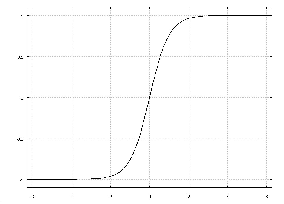
Figure 1: The Tanh() waveshaping function.
If we drive this function with a sinusoid input, we will be able to produce a nearly bandlimited signal. How bandlimited will depend on how hard we drive it, as higher input amplitudes will produce more and more harmonics, and take less advantage of its smoothing properties.
As with all types of waveshaping, the amplitude of the input signal will determine signal bandwidth, in a proportional way. If we want to keep a steady output amplitude, but vary the spectrum, we will need to apply an amplitude-dependent scaling. This is generally done by using a scaling function that takes the input amplitude as its argument and produces a gain that can be applied to the output signal. We can then refer to the amplitude of the input sinusoid as the distortion index.
The code for general-purpose waveshaping is based on standard function-mapping. It takes an input sinusoid, maps it using table lookup and then applies the required gain, also obtained through table lookup:
/* ar Waveshape kamp,kfreq,kndx,ifn1,ifn2,ifn3
   ifn1 is a sine/cosine
   ifn2 is the transfer function
   ifn3 is the scaling function
*/
opcode Waveshape,a,kkkiii

kamp,kf,kndx,isin,itf,igf  xin
asin oscili 0.5*kndx,kf,isin
awsh tablei asin,itf,1,0.5
kscl tablei kndx,igf,1
     xout awsh*kamp*kscl

endop
For hyperbolic waveshaping, we will need to provide two function tables, for the transfer (tanh) and the scaling functions, respectively:
f2 0 16385 "tanh" -157 157
f3 0  8193 4  2 1
The first Csound GEN draws tanh(x), over �p/50, and the second automatically generates a scaling function based on the previous table (2). To keep aliasing at bay, the index of distortion (kndx) can be estimated roughly as
kndx = 100/(kf*log10(kf))
If we would like to generate a sawtooth wave instead, we could take our square signal and apply the following expression:

(9)
By heterodyning it with a cosine wave, we can easily obtain the missing even components that make up the sawtooth signal. There will be a slight disparity in the amplitude of the second harmonic (about 2.5 dB), but the higher harmonics will be nearly as expected. This is a cheap way of producing a sawtooth wave.
opcode Sawtooth,a,kkkiii

 kamp,kf,kndx,isin,itf,igf  xin
 amod oscili  1,kf,1, 0.25
 asq Waveshape kamp*0.5,kf,kndx,isin,itf,igf
     xout  asq*(amod + 1)

endop
III. Asymmetrical FM synthesis
While the technique FM, and to a certain extent Phase Modulation (PM), too, synthesis are well known and have been explored in detail, some of its variants have not. One interesting method that seems to have been forgotten is the Asymmetrical FM method proposed by Palamin et al[9]. In their formulation, we have the original FM (or PM) model being ring-modulated by an exponentiated signal. This has the effect of introducing a new parameter that controls spectral symmetry that allows the peaks to be dislocated above or below the carrier frequency. Their expression (excluding a normalisation factor) is:

(10)
The new parameter r is the symmetry control, r < 1 pulling the spectral peak below the carrier frequency wc and r > 1 pushing it above. It is a very nice feature which can be added at the expense of a few multiplies and a couple of extra table lookups (for the cosine and the exponential). Note that what we have here is actually the ring modulation of a waveshaper output (using an exponential transfer function) and the FM signal. A nice way of tying up two distortion techniques together.
Implementing this is not too complicated. The exponential expression needs normalisation, which can be achieved by dividing it by exp(0.5k[r - 1/r]). When coding this, we will draw up an exponential table from 0 to an arbitrary negative value (say -50) and then look it up with a sign reversal (exp(-x)). This allows us to use the limiting table lookup mechanism in case we have an overflow. Since the values of exp() tend to have little variation for large negative values, limiting will not be problematic. In addition, to be faithful to the expression above (esp. in relation to component phases etc.), we will implement PM instead of FM:
/* ar Asfm kamp,kfc,kfm,kndx,kR,ifn1,ifn2,imax
   ifn1 is a sinewave
   ifn2 is an exp func between 0 and -imax
*/
opcode Asfm,a,kkkkkiii

 kamp,kfc,kfm,knx,kR,ifn,ifn2,imx xin
 kndx =  knx*(kR+1/kR)*0.5
 kndx2  = knx*(kR-1/kR)*0.5
 afm oscili  kndx/(2*$M_PI),kfm,ifn
 aph phasor  kfc
 afc tablei  aph+afm,ifn,1,0,1
 amod oscili kndx2, kfm, ifn, 0.25
 aexp tablei -(amod-abs(kndx2))/imx, ifn2, 1
    xout kamp*afc*aexp

endop
with the exponential function table (ifn2) drawn from 0 to -imx (-50):
f5 0 131072 "exp" 0 -50 1
In their original work, Palamin et al suggest a different method of normalisation. However, we found that it does not work for all values of r and k, for which the above method will generally do.
IV. PAF
One of the most recent new methods of distortion synthesis has been proposed by Miller Puckette in his PAF algorithm. In his paper[10], he starts with a desired spectral description and then works it out as ring-modulation of a sinusoid carrier and a complex spectrum (with low-pass characteristics). As his interest is to create formant regions, he will use the sinusoid to tune a spectral bump around a target centre frequency. The shape of the spectrum will be determined by his modulator signal, which in turn is generated by waveshaping using an exponentially-shaped transfer function. So we have PAF, in its simplest formulation, as:
(11)
Here, the waveshaper transfer function is f(x). The signal has a bandwidth B, a fundamental frequency at wm and its formant centre frequency is wc. This is in effect an implementation of one of Moorer's DSF equations (for double-sided, non-bandlimited spectra), cast in terms of cosines (instead of sines).
To this basic formulation, where we expect the wc to be an integer multiple of wm, a means of setting an arbitrary centre frequency is added. Instead of using a single carrier at wc, we will use two: one at wc1=n wm and another at wc2 =[n+1] wm. This will allow us to centre the formant at any frequency between the two carriers, by interpolating linearly between the two carrier signals. As a consequence, we will be able to sweep the formant frequency smoothly.
In addition, the complete PAF algorithm provides a 'frequency shift' parameter, which, if non-zero, allows for inharmonic spectra. This is effectively a phase modulation element, as seen in this more complete description of the method:
(12)
The complete Csound code of a more or less literal implementation of PAF is shown below:
opcode Func,a,a

asig xin
     xout  1/(1+asig^2)

endop


/* ar PAF kamp,kfun,kcf,kfshift,kbw,ifn
   ifn is a sine wave
*/
opcode PAF,a,kkkkki


kamp,kfo,kfc,kfsh,kbw,itb xin

kn = int(kfc/kfo)

ka = (kfc - kfsh - kn*kfo)/kfo

kg = exp(-kfo/kbw)

afsh phasor kfsh

 aphs phasor  kfo/2

a1 tablei 2*aphs*kn+afsh,1,1,0.25,1

a2 tablei 2*aphs*(kn+1)+afsh,1,1,0.25,1

asin tablei aphs, 1, 1, 0, 1

amod Func 2*sqrt(kg)*asin/(1-kg)

kscl = (1+kg)/(1-kg)

 acar = ka*a2+(1-ka)*a1
 asig = kscl*amod*acar
      xout asig*kamp

endop
The waveshaping here is performed by directly applying the function, since there are no GEN Routines in Csound which can directly generate such table. This is of course not as efficient as a lookup table, so there are two alternatives: writing a code fragment to fill a table with the transfer function, to be run before synthesis; or, considering that resulting distorted signal is very close to a Gaussian shape, use GEN20 to create one such wavetable. A useful exercise would be to reimplement the PAF generator above with table lookup waveshaping.
V. Modified FM synthesis
The final method we would like to present has been first briefly proposed by Moorer[4] in the 1970s, but lay dormant until we have re-discovered and explored some of its applications[16]. This technique has been named by us Modified FM synthesis (ModFM), as it is based on a slight change in the FM algorithm, with some important consequences.
An FM equation, when cast in complex exponential terms can look like this:

(13)
If we apply a change of variable z = -ik to the that formula, we will obtain the following expression:

(14)
which, is, when multiplied by the normalisation factor exp(-k), the basic Modified FM synthesis formula. One of the most important things about this algorithm is revealed by its expansion:

(15)
where In(k) are modified Bessel functions of the first kind, and constitute the basic (and substantial) difference between FM and ModFM. Their advantage is that they are (1) unipolar and (2) In(k) > In+1(k), which means that spectral evolutions are much more natural here. In particular, the scaled modified Bessels do not exhibit the much maligned 'wobble' seen in the behaviour of Bessel functions (see Figure 2). That very unnatural sounding characteristic of FM disappears in ModFM.
Figure 2: Scaled Modified Bessel functions orders 0 through 3
There are several applications of ModFM (as there are of FM) as well as small variations in its design. We will present here a basic straight implementation of the algorithm. Further examples and applications will be discussed in forthcoming articles. The Csound code uses, as in a previous example, table lookup to realise the exponential waveshaper in the ModFM formula. Apart from that, all we require is two cosine oscillators, yielding a very compact algorithm
/* ar ModFM kamp,kfc,kfm,kndx,ifn1,ifn2,imax
   ifn1 is a sine wave
   ifn2 is an exponential between 0 and -imax
*/
opcode ModFM,a,kkkkiii

 kamp,kfc,kfm,kndx,isin,iexp,imx xin
 acar oscili kamp,kfc,isin,0.25
 acos oscili 1,kfm,isin,0.25
 amod table  -kndx*(acos-1)/imx,iexp,1
     xout acar*amod

endop
With ModFM, it is possible to realise typical low-pass filter effects, by varying the index of modulation k. Also by using the carrier and modulation frequency as the centre of a formant and the fundamental, respectively, it is possible to reproduce the effect of a band-pass filter (and PAF). In fact a variant of the ModFM implementation above, with phase-synchronous signals can serve as a very efficient alternative to PAF and other formant synthesis techniques, such as FOF[17].
Final Words
In this article, a short tutorial on various distortion synthesis algorithms was offered. We have concentrated, particularly, on less well-known and more recent techniques. These methods have a common trait of offering elegant and low-cost solutions to the problem of generating complex time-varying spectra. They provide the sound designer an excelent alternative to other more computationally intensive and multi-parameter techniques. As an example of using the above methods, the following .csd file presents 7 simple instruments for MIDI performance using the UDOs discussed in the text.
<CsoundSynthesizer>
<CsOptions>
-dm0
</CsOptions>
<CsInstruments>

ksmps = 32
0dbfs = 1

opcode Blp,a,kkki
 setksmps 1
 ka,kf,kh,itb xin
 kn = int(sr/(2*kf))
 kn = int((kh > kn ? kn : kh))
 kph phasor kf/2
 kden tablei kph,itb,1
 if kden != 0 then
  knum tablei kph*(2*kn+1),itb,1,0,1
  asig = (ka/(2*kn))*(knum/kden - 1)
 else
  asig = ka
 endif
 xout asig
endop

opcode Blsum,a,kkkki
ka,kw,kt,kk,itb xin
kn = int(((sr/2) - kw)/kt)
aphw phasor kw
apht phasor kt
asin1 tablei aphw,itb,1
asin2 tablei aphw - apht,itb,1,0,1
asin3 tablei aphw + (kn+1)*apht,itb,1,0,1
asin4 tablei aphw + kn*apht,itb,1,0,1
acos  tablei apht,itb,1,0.25,1
kpw pow kk,kn+1
ksq = kk*kk
aden = (1 - 2*kk*acos + ksq)
asig = (asin1 - kk*asin2 - kpw*(asin3 - kk*asin4))/aden
knorm = sqrt((1-ksq)/(1 - kpw*kpw))
   xout asig*ka*knorm

endop

opcode NBlsum,a,kkkki
ka,kw,kt,kk,itb xin
aphw phasor kw
apht phasor kt
asin1 tablei aphw,itb,1
asin2 tablei aphw - apht,itb,1,0,1
acos tablei apht,itb,1,0.25,1
ksq = kk*kk
asig = (asin1 - kk*asin2)/(1 - 2*kk*acos + ksq)
knorm = sqrt(1-ksq)
   xout asig*ka*knorm
endop

opcode Waveshape,a,kkkiii
kamp,kf,kndx,isin,itf,igf  xin
asin oscili 0.5*kndx,kf,isin
awsh tablei asin,itf,1,0.5
kscl tablei kndx,igf,1
     xout awsh*kamp*kscl
endop

opcode Sawtooth,a,kkkiii
kamp,kf,kndx,isin,itf,igf  xin
amod oscili  1,kf,1, 0.25
asq Waveshape kamp*0.5,kf,kndx,isin,itf,igf
     xout  asq*(amod + 1)
endop


opcode Asfm,a,kkkkkii
kamp,kfc,kfm,knx,kR,ifn,ifn2 xin
kndx =  knx*(kR+1/kR)*0.5
kndx2  = knx*(kR-1/kR)*0.5
afm oscili  kndx/(2*$M_PI),kfm,ifn
aph phasor  kfc
afc tablei  aph+afm,ifn,1,0,1
amod oscili kndx2, kfm, ifn, 0.25
aexp tablei (abs(kndx2) - amod)/50, ifn2, 1
   xout kamp*afc*aexp;exp(amod - abs(kndx2/2))
endop


opcode Func,a,a
asig xin
     xout  1/(1+asig^2)
endop

opcode PAF,a,kkkkki
 kamp,kfo,kfc,kfsh,kbw,itb xin
 kn = int(kfc/kfo)
 ka = (kfc - kfsh - kn*kfo)/kfo
 kg = exp(-kfo/kbw)
 afsh phasor  kfsh
 aphs phasor  kfo/2
 a1  tablei  2*aphs*kn+afsh,1,1,0.25,1
 a2  tablei  2*aphs*(kn+1)+afsh,1,1,0.25,1
 asin  tablei  aphs, 1, 1, 0, 1
 amod Func 2*sqrt(kg)*asin/(1-kg)
 kscl = (1+kg)/(1-kg)
 acar = ka*a2+(1-ka)*a1
 asig = kscl*amod*acar
      xout asig*kamp
endop

opcode ModFM,a,kkkkiii
kamp,kfc,kfm,kndx,isin,iexp,imx xin
acar oscili kamp,kfc,isin,0.25
acos oscili 1,kfm,isin,0.25
amod table -kndx*(acos-1)/imx,iexp,1
     xout acar*amod
endop

instr 1  /* MIDI channel 1, bandlimited pulse */

kfr  cpsmidib 2
iamp ampmidi 1
kh   midic7 1,1,100

asig Blp iamp,kfr,kh, 1
aout linenr asig*0.2,0.01,0.1,0.01
      out aout
endin

instr 2  /* MIDI channel 2, bandlimited DSF */

kfr  cpsmidib 2
iamp ampmidi 1
kk   midic7 1,0.001,0.999
kra  midic7 91,0.5,2
kk port kk, 0.01
asig Blsum iamp,kfr,kfr/kra,kk,1
aout linenr asig*0.2,0.01,0.1,0.01
      out aout
endin

instr 3  /* MIDI channel 3, non-bandlimited DSF */

kfr  cpsmidib 2
iamp ampmidi 1
kk   midic7 1,0.001,0.99
kra  midic7 91,0.25,1

kk port kk, 0.01
asig NBlsum iamp,kfr,kfr/kra,kk,1
aout linenr asig*0.2,0.01,0.1,0.01
      out aout

endin

instr 4  /* MIDI channel 4, waveshaping (saw & square) */

kfr  cpsmidib 2
iamp ampmidi 1
kk   midic7 1,0.001,0.99
kra  midic7 91,0,1

kk port kk, 0.01
asig1 Sawtooth iamp,kfr,kk,1,2,3
asig2 Waveshape iamp,kfr,kk,1,2,3
aout  linenr (kra*asig1 + (1-kra)*asig2)*0.2,0.01,0.1,0.01
      out aout
endin

instr 5 /* MIDI channel 5, Asymmetric FM */

kfr  cpsmidib 2
iamp ampmidi 1
kk   midic7 1,0,15
kra  midic7 91,1,2
kR   midic7 93,0.5,2

kk port kk, 0.01
kR port kR, 0.01
asig Asfm iamp,kfr,kfr/kra,kk,kR,1,5
aout linenr asig*0.2,0.01,0.1,0.01
      out aout
endin

instr 6 /* MIDI channel 6, PAF */

kfr  cpsmidib 2
iamp ampmidi 1
kQ   midic7 1,1,10
kfor  midic7 91,900,2800
ksh   midic7 93,0,100

kQ port kQ, 0.01
ksh port ksh, 0.01
asig PAF iamp,kfr,kfor,ksh,kfor/kQ,1
aout linenr asig*0.05,0.01,0.1,0.01
      out aout
endin

instr 7 /* MIDI channel 7, Modified FM */

kfr  cpsmidib 2
iamp ampmidi 1
kk   midic7 1,0,25
kra  midic7 91,0.25,1

kk port kk, 0.01
asig ModFM iamp,kfr,kfr/kra,kk,1,5,50
aout linenr asig*0.2,0.01,0.1,0.01
      out aout

endin

</CsInstruments>

<CsScore>
f1 0 16384 10 1
f2 0 16385 "tanh" -157 157
f3 0  8193 4  2 1
f4 0 16385 -12 50
f5 0 131072 "exp" 0 -50 1

f0 36000

e
</CsScore>
</CsoundSynthesizer>
Acknowledgements
This research was partly funded by a grant from An Foras Feasa, the Humanities Institute, NUI, Maynooth. An earlier version of this article was presented at the Linux Audio Conference, 2009.
References
[1] Chowning, J. 1973,"The Synthesis of Complex Audio Spectra by Means of Frequency Modulation." Journal of the Audio Engineering Society (21): 526-34.
[2] Windham, G. and K. Steiglitz 1970, “Input Generators for Digital Sound Synthesis”. Journal of the Acoustic Society of America, 47(2): 665-6.
[3] Moorer, J. A. 1976,“The Synthesis of Complex Audio Spectra by Means of Discrete Summation Formulas”. Journal of the Audio Engineering Society, 24 (9).
[4] Moorer, J. A. 1977,“Signal Processing Aspects of Computer Music: A Survey”, Proceedings of the IEEE, 65 (8): 1108 – 1141.
[5] Arfib, D. 1978,“Digital Synthesis of Complex Spectra by Means of Multiplication of Non-Linear Distorted Sinewaves”. AES Preprint No.1319 (C2).
[6] Le Brun, M. 1979,“Digital Waveshaping Synthesis”. Journal of the Audio Engineering Society, 27(4): 250-266.
[7] Schottstaedt, W. 1977, “ The Simulation of Natural Instrument Tones Using a Complex Modulating Wave”. Computer Music Journal 1(4): 46-50.
[8] Le Brun, M. 1977,“A Derivation of the Spectrum of FM with a Complex Modulating Wave”, Computer Music Journal, 1(4):51-52
[9] Palamin, J.P., P. Palamin and A. Ronveaux 1988,”A Method of Generating and Controlling Musical Asymmetric Spectra”. Journal of the Audio Engineering Society 36 (9): 671-685
[10] Puckette, M. 1995, "Formant-Based Audio Synthesis Using Nonlinear Distortion." Journal of the Audio Engineering Society 43(1): 40-47.
[11] Lazzarini, V., J. Timoney and T. Lysaght 2008,“Split-Sideband Synthesis”. Proceedings of the ICMC 2008, Belfast, UK,
[12] Lazzarini, V., J. Timoney and T. Lysaght 2007,“Adaptive FM synthesis”. Proceedings of the 10th Intl. Conference on Digital Audio Effects (DAFx07). Bordeaux: University of Bordeaux: 21-26.
[13] Lazzarini, V., J. Timoney and T. Lysaght 2008,“The Generation of Natural-Synthetic Spectra by Means of Adaptive Frequency Modulation”. Computer Music Journal, 32 (2): 12-22.
[14] Lazzarini, V., J. Timoney and T. Lysaght 2008,“Asymmetric Methods for Adaptive FM Synthesis”. Proceedings of the International Conference on Digital Audio Effects, Helsinki, Finland.
[15] Cabrera, A. (Ed.). The Csound Manual. http://csounds.com/manual.
[16] Lazzarini, V., J. Timoney, 2008, "New Perspectives on Distortion Synthesis for Virtual Analogue Oscillators". Submitted to Computer Music Journal.
[17] Rodet, X. 1984. “Time Domain Formant-Wave-Function Synthesis”. Computer Music Journal, 8 (3):9-14.